2-Point Perspective: Precision Method

My perspective drawings typically involve two vanishing points that are located well off the page to either side. The methods that I found for working in such a system were unsatisfying, as they (a) relied on interpolation by eye, and (b) involved drawing grid lines on the paper. The former is problematic, because interpolating by eye is inexact and can result in major errors when spanning large distances. The latter is problematic because it not only clutters up the drawing space, but the lines can become confusing as the drawing fills in and furthermore can be difficult to fully erase. This led me to developing a system based on the grid method, but using trigonometry to make the lines to the vanishing points precise. To see how the grid method works, the book “How to Draw” by Scott Robertson (Chapter 4: Creating Grids – The Brewer Method) has a good summary.

The steps for my method can be broken down as follows:

Step 1: Conceptualize the space to be represented in 3D,
Step 2: Define the conceptual lines in space using linear equations,
Step 3: Use the linear equations as a means to locate the horizon line, and left and right vanishing points,
Step 4: Develop equations for use in projecting a line from any point on the page to the right or left vanishing point.

The majority of the work occurs in Step 2 and Step 3. The bad news is that these steps are a bit labour-intensive. The good news is that these steps need only be done once.

Overview of Method

In the end, the objective of this method is to define the Horizon Line, the Left Vanishing Point (LVP) and the Right Vanishing Point (RVP) in a Cartesian coordinate system, with the bottom left corner of the paper acting as the origin point (0,0). In this system, any point on the page can be assigned a coordinate by measuring (in cm) its location horizontally and vertically from (0,0). With the LVP and RVP also defined as Cartesian coordinates relative to (0,0), a line drawn between the point of interest and the vanishing point becomes the hypotenuse of a right-angle triangle with the Horizon Line (see Figure 6 below). Applying this method, you can determine the angle from the point of interest to the desired vanishing point, and use a protractor positioned at the point of interest to draw it out.

Step 1: Conceptualize the 3D space

The method starts with drawing four lines to define the space to be represented: one vertical line, two lines that converge to a hypothetical vanishing point in one direction, and one line towards the opposite vanishing point – see Figure 1. This is the same first step as in the gridding method, per the Robertson book noted above. Imagine this as being a box that will eventually contain your drawing.

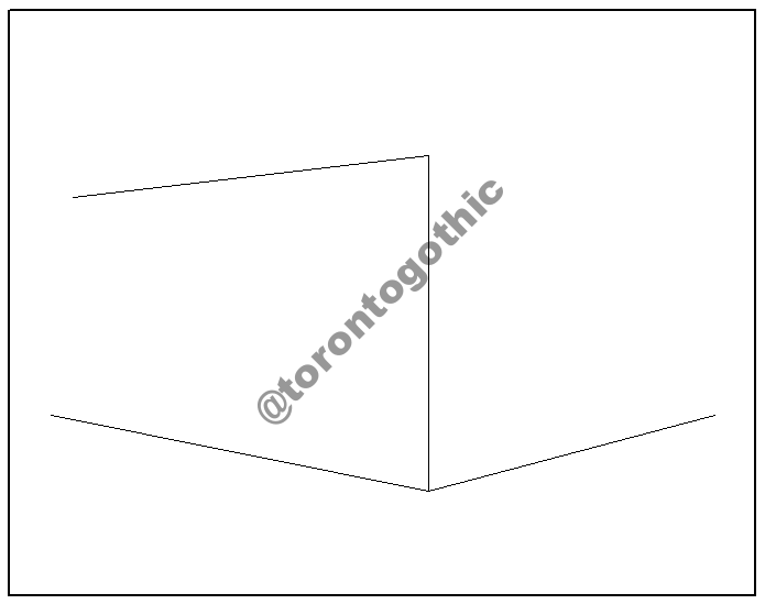
Figure 1: Start by drawing a vertical line. Imagine the object you will be drawing as being contained within a box and this vertical line is the front edge. At the top and bottom, draw two lines going to the left that will converge somewhere off of the page. Again from the bottom, draw a line going to the right towards where you imagine the right vanishing point would be. You can see that this resembles part of a cube – imagine your drawing sitting within it.

Step 2: Define the lines in 2D

The next step will be to define these lines in 2D space, in a Cartesian coordinate system with the bottom left corner of the page as the origin (0,0). The lines are to be defined in terms of their slope (m) and y-intercept (b) as per the form of the linear equation y = mx + b. Recalling high school algebra, the slope is the rise over the run of the line, and the y-intercept is the location at which is passes the y-axis (the left side of the paper in this method).

2a: Slope of Line 1

The slope can be determined by measuring horizontally some distance (the length doesn’t matter – choose a round number to make things easier) and the corresponding distance vertically, as shown in Figure 2.

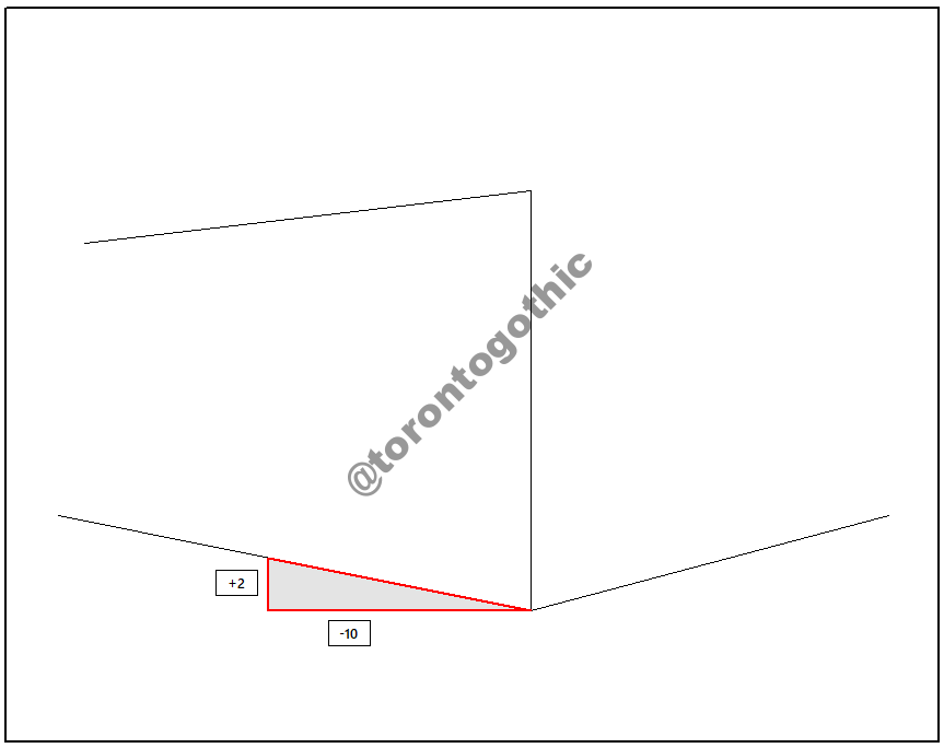
Figure 2: To get the slope of the bottom line going to the left, I measured back 10 cm (run of -10), and the corresponding height to meet the line was 2 cm (rise of +2). Therefore, the slope is:

m = rise/run = (+2)/(-10) = -0.2

2b: Y-intercept of Line 1

The y-intercept is determined by plugging an (x,y) coordinate pair from the line into the linear equation, with the slope calculated above. The linear equation rearranged to solve for b is: b = y – mx. A coordinate pair on the line can be determined by measuring from the bottom left corner of the page, as shown in Figure 3.

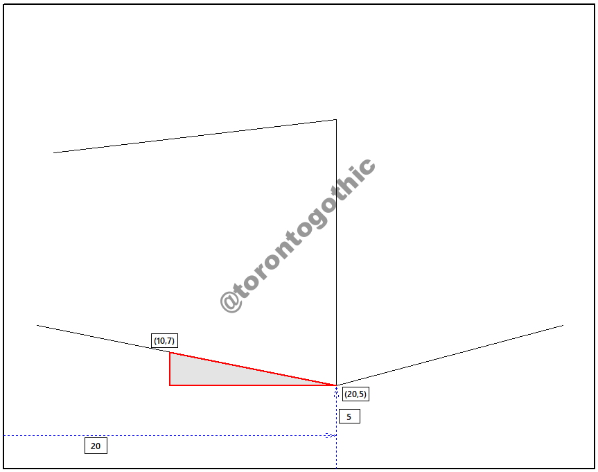
Figure 3: The first point of the line is shown here to be at an (x,y) coordinate pair of (20,5) as measured from the bottom left corner of the page. If we plug that into the equation b = y – mx using the slope (m) of -0.2 as calculated in Figure 2, the resulting value for b is:

b = y – mx = 5 – (-0.2)(20) = 9.

This means that if the line were continued until it passed the y-axis (the left side of the page), it would cross at a height of 9 cm above the bottom of the page. It can be see that subbing in a different coordinate pair will, as would be expected, result in the same number:

b = y – mx = 7 – (-0.2)(10) = 9

Thus, this line, we’ll call Line 1, is defined by the equation:

y = -0.2x + 9

2c: Slope and y-intercept for Line 2

The next step is to do the same thing for the other line that is going to the left. This is shown in Figure 4.

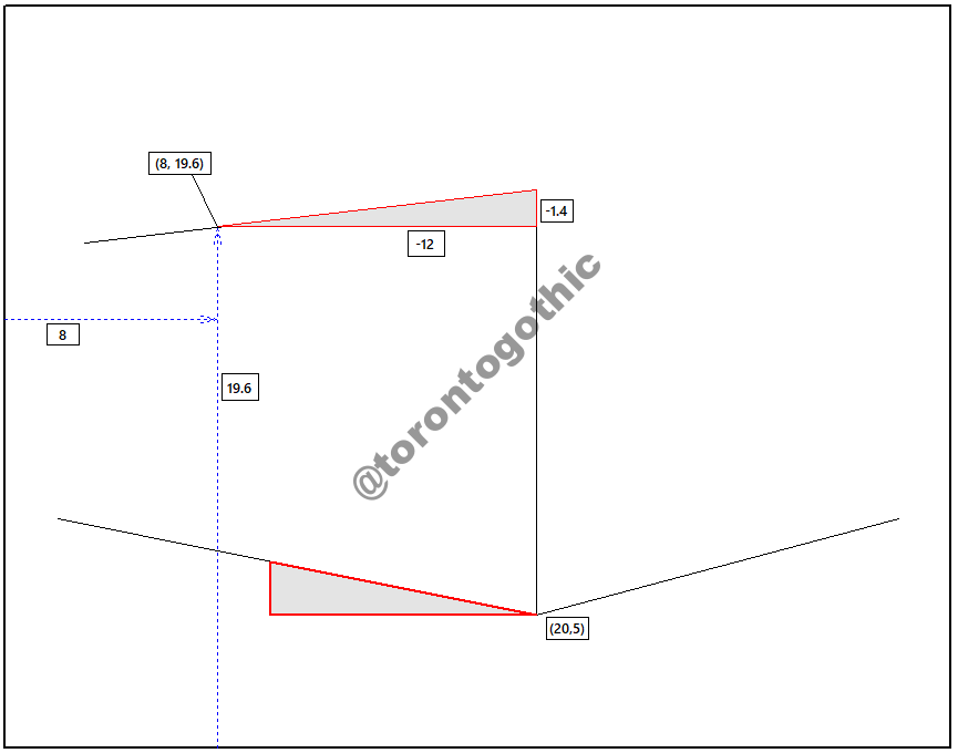
Figure 4: I have pre-filled some values here using the same approach as before. The “run” is a random measurement of -12 cm, which has a corresponding “rise” of -1.4 cm. This results in a slope of m = 0.1167.

Subbing a point along the line into the equation of b = y – mx gives a y-intercept value of 19.6 – (0.1167)(8) = 18.7 (in other words, if the line as-drawn continued, it would cross the y-axis, or the left side of the page, at 18.7 cm above the origin point, or the bottom left corner).

So this line, we’ll call Line 2, is defined by the equation:

y = 0.1167x + 18.7

Step 3: Identify the Horizon Line and Vanishing Points

3a: Define the Horizon Line and LVP Location

By definition, the vanishing points occur on the horizon line. As such, we know that the y-coordinate where Line 1 and Line 2 converge will be the location of the horizon line. This is shown conceptually in Figure 5.

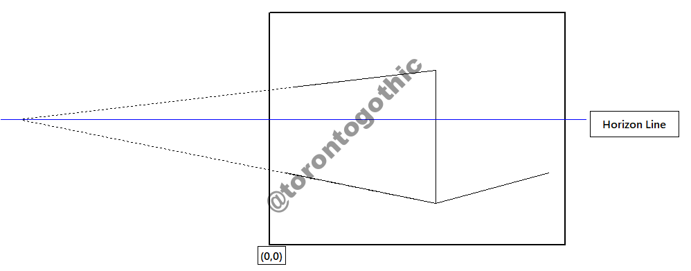
Figure 5: The y-coordinate where the lines converge will represent the height of the horizon line (above the bottom of the paper).

In other words, the horizon line will occur at the location where the “y” value of Line 1 and Line 2 are the same. Recalling the equations above:

Line 1: y1 = -0.2(x1) + 9

Line 2: y2 = 0.1167(x2) + 18.7

The horizon line occurs where y1 = y2, or:

-0.2(x1) + 9 = 0.1167(x2) + 18.7

At this point, the two lines will share an x-coordinate as well (i.e., x1 = x2) and the equation can be rearranged to solve for x:

x = (18.7 – 9)/(-0.2 – 0.1167) = -30.6

This can be subbed into either of the equations to get the corresponding y value:

y = (0.1167)(-30.6) + 18.7 = 15.1

So the horizon line occurs at 15.1 cm above the bottom of the page, as shown in Figure 6, and the coordinate of the Left Vanishing Point (LVP) is: LVP = (-30.6, 15.1).

KEY EQUATIONS

The equations in general terms (i.e., m1 and b1 for the slope and intercept of Line 1, and m2 and b2 for the slope and intercept of Line 2) are:

x = (b2 – b1)/(m1 – m2), and

y = m1x + b1 or m2x + b2

Figure 6: This shows the location of the LVP in terms of coordinates relative to the bottom left corner of the page.

3b: Define the RVP Location

Now that we know the horizon line is at a height of 15.1 cm above the bottom of the page, we know that will be the height where the Right Vanishing Point (RVP) resides. All we need then is the associated x-coordinate. This is done by determining the slope and intercept as was done for Line 1 and Line 2, then subbing 15.1 in as the y-coordinate to get the associated x-coordinate. This is done in Figure 7.

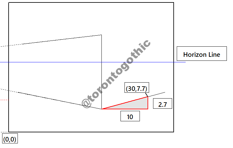
Figure 7: The slope and y-intercept are calculated as before. The rise is 2.7 cm and the run is 10 cm for a slope of 0.27. The y-intercept is calculated using a coordinate pair from the line, in this case (30,7.7) was measured off, resulting in b = y – mx = -0.4 (i.e., if the line were continued to the left, it would cross the y-axis, or left side of the page, at -0.4).

The equation that defines this line is therefore y = 0.27x – 0.4

The line going to the right was shown in Figure 7 to be defined by the equation y = 0.27x – 0.4. If we solve for x after subbing in a y-value of 15.1 (the height of the horizon line) we get a value of 57.4, meaning that the line will converge with the horizon at 57.4 cm from the left side of the page, as shown in Figure 8.

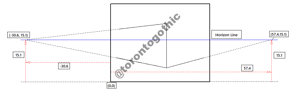
Figure 8: This figure shows how subbing in the horizon line height to the linear equation defining the line going to the right gives the x-coordinate of the RVP.

Step 4: Derive Equations for Protractor Angles

At this point, we now know the locations of the LVP and RVP as distances relative to the bottom corner of the paper. Now, any point on the paper will form a right-angled triangle with the LVP or RVP and the horizon line. As such, the angle from the desired point to the horizon line can be calculated, so that a protractor can be used to plot it and draw it in practice.

4a: Line to RVP

An example is shown in Figure 9. In this case, we want to draw a line from a given point on the page to the RVP. The point has been measured from the bottom left corner of the page and has a coordinate (17,6).

Figure 9: Here we have a point at (17,6) and we want to know the angle that we would need to measure from a protractor to get a line to the RVP (theta*). Note that theta and theta* are equivalent, and this angle can be calculated using the trigonometric ratio tan(theta) = opposite/adjacent. The opposite and adjacent distances can be calculated based on the coordinates, as shown. The opposite distance is the height of the horizon line minus the y-coordinate of the point of interest (9.1) and the adjacent distance is the x-coordinate of the RVP minus the x-coordinate of the point of interest (40.4). The value of theta (and therefore theta*) is the inverse tan of 9.1/40.4, or 12.7 degrees.

As shown in Figure 9, when measuring to the RVP, the equation in general terms is:

theta* = tan^-1(opp./adj.) = tan^-1((RVPy – y)/(RVPx – x)),

where RVPx and RVPy are the x and y coordinates of the RVP, respectively, and x and y are the coordinates of the point of interest.

2b: Line to the LVP

Measuring to the LVP requires crossing the y-axis and so the equation is slightly different, as illustrated in Figure 10, using the same point of interest (17,6).

Figure 10: For the LVP, the calculation of the opposite length is the same (LVPy – y), or 9.1 for this example. For the adjacent length, is the x-coordinate of the LVP (LVPx) as a positive number, plus the x-coordinate of the value of interest, or -LVPx + x.

Per Figure 10, the angle measured by protractor to the LVP is (in general terms):

theta* = tan^-1(opp./adj.) = tan^-1((LVPy – y)/(-LVPx + x))

For this example, the angle is 10.8 degrees.

Once you have the coordinates for the LVP and RVP, you can use the above equations to measure off the exact angle from any point on the page. This is the method I’ve used for all of my recent perspective drawings.